If you are working in tech and you aren’t building a RAG app at your company, it’s likely that you know colleagues who are. The key part of any RAG app is finding documents (or parts of documents) that are relevant to the user’s query and could be used as part of an LLM context to answer this query accurately. So far the best way we’ve found of finding these relevant documents is vector search.
Vector search finds relevant documents by converting both documents and queries into high-dimensional numerical vectors (embeddings) that capture semantic meaning. Instead of matching exact keywords like traditional search, vector search finds documents that are conceptually similar. When you search for “machine learning optimization,” it can find documents about “neural network tuning” or “AI model improvement” even if they don’t contain your exact terms.

The vector search process involves several key steps:
- Document ingestion - Starting with raw text content that needs to be searchable
- Calculating embeddings - Converting text into high-dimensional vectors using embedding models
- Storing - Saving these vectors in a specialized vector database optimized for similarity search
- Querying - Converting user search queries into vectors using the same embedding model
- Finding similar docs - Calculating distances between the query vector and stored vectors to identify matches
- Returning results - Returning the most relevant documents ranked by similarity score
The process splits into two phases: indexing (steps 1-3) done once during setup, and querying (steps 4-6) executed in real-time for each search. This lets you find documents that mean the same thing, not just ones with the exact same words - when you search for “machine learning optimization,” it can find documents about “neural network tuning” even without matching terms.
The internet is full of tutorials and examples of how to get started with the vector search and vector databases. The examples work great for ~10k documents on your laptop, but production changes everything. Suddenly you’re looking at hundreds/thousands $$ in cloud bills and search latency isn’t what you were used to when playing with a toy dataset of documents. In this post, we won’t be covering the basics and we’ll assume certain level of familiarity with the concept of vector search. Here we’ll focus on the real-world challenges of scaling vector search to production: managing costs, optimizing distributed workloads, and building systems that handle millions of documents without the ballooning costs.
To showcase this approach, we’ve built a vector search system over 1M documents using RedisVL and SkyPilot:
- SOTA embedding model
- 1M documents
- Total indexing cost: $0.85
- Query latency: sub-100ms
- No Kubernetes or no complex pipelines.
The scale problems most tutorials skip
Vector database tutorials cover the basics well, but miss the problems that surface at scale:
Bigger GPUs aren’t a panacea: processing 1M documents on a single GPU could easily take a few hours. Using a bigger GPU just makes it more expensive, but not much faster.
Distributed work gets complicated: introducing parallel processing by using multiple machines is a good idea, but it often means building job schedulers, handling partial failures, and debugging mysterious worker crashes during document 847,392.
Query latency degrades at scale: That snappy 10ms response time with 10k documents becomes 500ms+ with millions of documents, making your application feel sluggish and unresponsive.
Scaling vector databases requires orchestration, performance, and cost optimization. We’ve chosen the RedisVL + SkyPilot combination to address these problems.
Why RedisVL + SkyPilot works
After having worked with various vector databases and orchestration tools, this setup addressed issues that individual tools couldn’t:
Direct streaming eliminates data movement Most architectures use extract -> compute -> store -> load. Our approach streams compute results directly to Redis. No intermediate files, no S3 buckets, no wondering about worker completion status.
This combination makes scaling easy SkyPilot can quickly spin up hundreds of workers across multiple clouds, while RedisVL can comfortably ingest thousands of vector embeddings per second with its optimized batch loading capabilities.
RedisVL’s performance edge
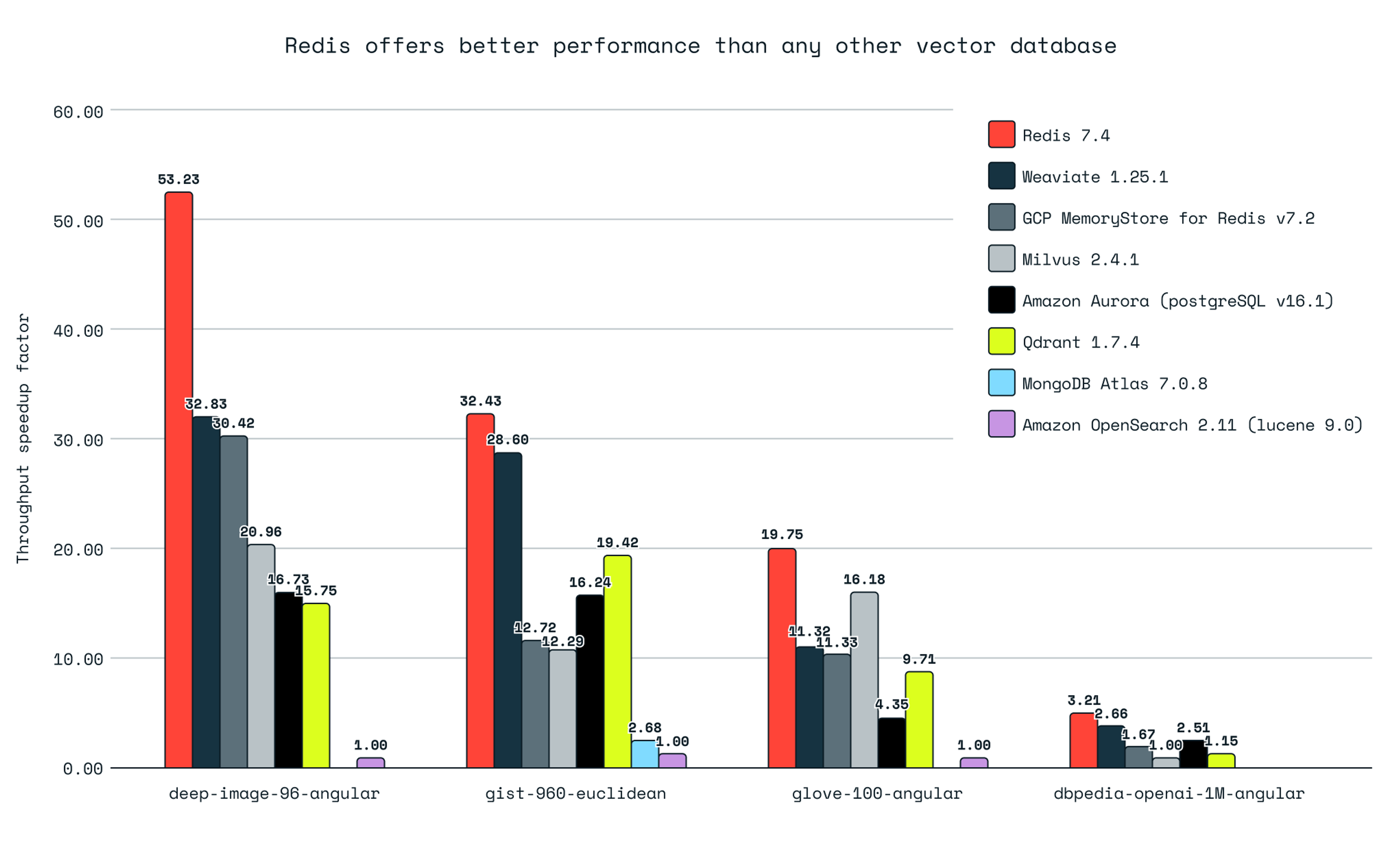
The benchmarks show RedisVL is pretty fast. Redis achieved up to 3.4 times higher queries per second (QPS) than Qdrant, 3.3 times higher QPS than Milvus, and 1.7 times higher QPS than Weaviate for the same recall levels (source). But raw speed isn’t the only advantage - hybrid query capabilities matter more in practice.
RedisVL excels at complex filtering A lot of other vector databases handle “find similar documents” well but struggle with “find papers from 2020-2024 published at NeurIPS that are similar to this query.” RedisVL lets you write (@year:[2020 2024] @venue:{NeurIPS}) => [KNN 10 @paper_embedding $vec] and it executes efficiently.
RedisVL simplifies working with vectors in Redis. It provides abstractions and utilities to help you store, index, and query vectors efficiently, supporting advanced features like indexing multiple fields in Redis hashes and JSON, vector similarity search with HNSW, FLAT or SVS-VAMANA algorithms, and vector range search.
RedisVL was designed as a search engine that excels at vectors. When searching “wireless headphones under $100 with good reviews,” you’re combining semantic understanding with structured filters. Redis includes a high-performance vector database that lets you perform semantic searches over vector embeddings. You can augment these searches with filtering over text, numerical, geospatial, and tag metadata.
SkyPilot’s scalability advantages
SkyPilot simplifies distributed computing: Normally, splitting work across multiple GPUs requires custom job schedulers, failure handling, and data partition management. SkyPilot reduces all of this to a YAML file with automatic retries. Spot instance gets preempted? Job restarts on a different cloud. Can’t find T4s on AWS? Tries GCP. No available spots? Falls back to on-demand.
Multi-cloud strategies are essential for modern AI workloads: There are now way more cloud providers than just AWS, GCP, and Azure. The AI neocloud ecosystem has exploded with specialized GPU providers like Nebius and Lambda Labs offering significantly better pricing on high-end GPUs (H100, H200), while established clouds excel at providing older GPU types (T4, A10, L4, V100) with broader availability. Different clouds have different availability and pricing, so using multiple clouds helps you get cheaper, more reliable access to GPUs.

SkyPilot delivers practical multi-cloud benefits: Companies using this in production are seeing real cost savings and getting more done. Salk Institute’s scientists reduced their brain mapping computation costs by 6.5x using SkyPilot’s Managed Spot across hundreds of instances (sources: 1 and 2). But it’s not just about saving money - SkyPilot removes all the annoying ops work that usually kills distributed computing projects - automatically finding the cheapest available resources across all your cloud accounts and handling the complexity of multi-cloud orchestration.
The architecture that scales

Each worker:
- Downloads its assigned chunk of the dataset (e.g. 200k documents per worker when using 5 workers)
- Generates embeddings using sentence-transformers
- Streams results directly to Redis using RedisVL’s bulk loading
- Automatically retries on failure, picks up exactly where it left off
Zero coordination between workers. No shared storage. No complex failure recovery. Just simple parallel compute.
The numbers
Here’s the actual cost breakdown:
Embedding generation (1M documents)
- Hardware: T4/L4/A10G spot instances (configurable in YAML)
- Cost estimate: ~$0.85 with T4 spot instances
- Model:
nomic-ai/nomic-embed-text-v2-moe(768 dimensions, truncatable to 256)
Search performance & cost breakdown
The $0.85 indexing cost breaks down as follows:
T4 spot @ $0.13/hour × 5 instances × 1.3 hours = $0.85
Why scaling matters: faster results at the same cost
Here’s the thing: running jobs in parallel lets you finish the same work much faster for the same price. When you scale horizontally across multiple instances, you’re essentially trading sequential time for parallel execution. This means:
- Faster time-to-insight: Get your vector index ready in minutes instead of hours
- Same budget, better performance: Cloud providers charge by instance-hour, so 10 instances for 1 hour costs the same as 1 instance for 10 hours
- Better resilience: If one instance fails, others continue processing
Here’s how scaling impacts performance while maintaining the same ~$0.85 budget:
| Number of Instances | Time to Index 10K Papers (Processing Only) | Cost | Speedup |
|---|---|---|---|
| 1 | ~400 minutes (~6.5h) | $0.85 | 1x |
| 5 | ~80 minutes (~1.3h) | $0.85 | 5x |
| 10 | ~40 minutes (~0.67h) | $0.85 | 10x |
Some notes:
These times reflect processing time only. Instance startup and dependency installation add another 5-7 minutes. You can minimize this overhead by using custom Docker images with SkyPilot that have dependencies pre-installed.
Your numbers might vary based on instance availability, network latency, and Redis cluster performance.
If you are ok using a smaller embedding model, you can bring the cost down to mere cents (a bit more on that below).
This is where SkyPilot shines as the best way to scale: it handles the orchestration complexity, manages spot instance failures, and ensures your jobs complete successfully across any cloud provider.
Implementation: the tricky parts
The complete system includes:
- API: FastAPI service with Streamlit UI
- Query functionality: Hybrid vector similarity + traditional filters
- Data: Research papers with metadata (title, abstract, authors, venue, year)
Distributed embedding jobs: smart workload distribution
This section shows how we implement the Distributed Embedding Jobs component from our architecture. Naive chunking creates unbalanced loads. With the below approach, we ensured that every worker gets roughly equal work across our 5x GPU spot instances.
def calculate_job_range(total_records, job_rank, total_jobs):
    """Distribute records evenly, handling remainder properly"""
    chunk_size = total_records // total_jobs
    remainder = total_records % total_jobs

    # Jobs 0 to remainder-1 get one extra record
    job_start = job_rank * chunk_size + min(job_rank, remainder)
    if job_rank < remainder:
        chunk_size += 1

    return job_start, job_start + chunk_size

# Launch distributed jobs
for job_rank in range(5):
    start_idx, end_idx = calculate_job_range(1000000, job_rank, 5)

    task = sky.Task.from_yaml('embedding_job.yaml')
    task.update_envs({
        'JOB_START_IDX': str(start_idx),
        'JOB_END_IDX': str(end_idx),
    })

    # SkyPilot handles cloud selection, spot instances, retries
    sky.jobs.launch(task)
Here’s what the launch looks like in practice:
$ python batch_embedding_launcher.py --num-jobs 5 --env-file .env
Launched job for records 0-200000
Launched job for records 200000-400000
Launched job for records 400000-600000
Launched job for records 600000-800000
Launched job for records 800000-1000000

5 jobs launched successfully!
You can monitor the distributed jobs with SkyPilot’s job queue:
$ sky jobs queue
Fetching managed job statuses...
Managed jobs
In progress tasks: 5 STARTING
ID  TASK  NAME            REQUESTED                                       SUBMITTED   TOT. DURATION  JOB DURATION  #RECOVERIES  STATUS     WORKER_POOL
14  -     embeddings-job  1x[T4:1, V100:1, A10G:1, L4:1][On-demand|Spot]  1 min ago   1m 14s         -             0            STARTING   None
13  -     embeddings-job  1x[A10G:1, T4:1, V100:1, L4:1][On-demand|Spot]  1 min ago   1m 43s         -             0            STARTING   None
12  -     embeddings-job  1x[L4:1, V100:1, A10G:1, T4:1][On-demand|Spot]  2 mins ago  2m 11s         -             0            STARTING   None
11  -     embeddings-job  1x[T4:1, V100:1, L4:1, A10G:1][On-demand|Spot]  2 mins ago  2m 42s         -             0            STARTING   None
10  -     embeddings-job  1x[T4:1, V100:1, L4:1, A10G:1][On-demand|Spot]  3 mins ago  3m 7s          -             0            STARTING   None
Notice how SkyPilot automatically tries different GPU types based on availability. Each job specifies multiple acceptable GPUs (T4, L4, A10G, V100) and SkyPilot picks whichever is available and cheapest.
Here’s the GCP Compute dashboard showing the 5 instances provisioned by SkyPilot for parallel processing:

Each job processes its chunk of documents independently. Here’s what the execution looks like:
$ sky jobs logs 14
...
(setup pid=4198) Unzipping dataset...
(setup pid=4198) Archive:  data/research-papers-dataset.zip
(setup pid=4198)   inflating: data/dblp-v10.csv
(setup pid=4198) Dataset ready at data/dblp-v10.csv
(embeddings-job, pid=4198) Processing papers: Records 800000-1000000
(embeddings-job, pid=4198) 12:23:42 __main__ INFO   Processing records 800000-1000000 of 1000000
(embeddings-job, pid=4198) 12:23:42 redisvl.index.index INFO   Index already exists, not overwriting.
(embeddings-job, pid=4198) 12:23:42 __main__ INFO   Created new Redis index
(embeddings-job, pid=4198) 12:23:43 sentence_transformers.SentenceTransformer INFO   Use pytorch device_name: cuda:0
(embeddings-job, pid=4198) 12:23:43 sentence_transformers.SentenceTransformer INFO   Load pretrained SentenceTransformer: nomic-ai/nomic-embed-text-v2-moe
Batches: 100%|██████████| 320/320 [00:08<00:00, 35.90it/s]
Batches: 100%|██████████| 320/320 [00:17<00:00, 17.90it/s]
(embeddings-job, pid=4198) Records 800000-1000000:  10%|█         | 20480/200000 [00:29<04:31, 661.40it/s]
(embeddings-job, pid=4198) Batches:  17%|█▋        | 54/320 [00:04<00:19, 13.53it/s]
The logs show the full pipeline: dataset download, index creation, model loading, and batch processing with real-time progress. Each worker handles 200,000 documents independently (1M / 5 workers), streaming results directly to Redis.
Direct stream to Redis: pipeline with backpressure
This implements the Direct Stream to Redis component from our architecture, where RedisVL manages ingestion. Overlapping compute and I/O improves throughput While the GPU generates embeddings for batch N+1, Redis ingests batch N. This keeps the GPU busy - while it’s working on one batch, Redis is saving the previous batch.
def redis_writer(queue, index):
    """Background thread that streams batches to Redis"""
    while True:
        batch = queue.get()
        if batch is None:
            break
        try:
            index.load(batch, id_field='id')
            logger.info(f"Streamed {len(batch)} papers to Redis")
        except Exception as e:
            logger.error(f"Redis write failed: {e}")
        queue.task_done()

# producer-consumer with bounded queue for backpressure
redis_queue = Queue(maxsize=10)  # prevent potential memory explosion
writer_thread = Thread(target=redis_writer, args=(redis_queue, index))
writer_thread.start()

# generate embeddings and stream to Redis
for batch in process_papers_in_batches(papers, batch_size=256):
    embeddings = model.encode([p['abstract'] for p in batch])

    processed = [
        {
            'id': f"paper:{paper['id']}",
            'title': paper['title'],
            'abstract': paper['abstract'],
            'authors': paper['authors'],
            'venue': paper['venue'],
            'year': safe_int(paper['year']),
            'paper_embedding': embedding.astype(np.float32).tobytes()
        }
        for paper, embedding in zip(batch, embeddings)
    ]

    redis_queue.put(processed)
As workers stream data to Redis, you can monitor performance metrics in real-time through the Redis Cloud dashboard:

FastAPI search service: production-ready API
This is our FastAPI Search Service implementation from the architecture (plus a demo Streamlit app). Hybrid queries combine semantic search with traditional filtering in a single operation. This works better than vector databases that don’t prioritize filtering.
@app.post("/search", response_model=SearchResponse)
async def search_papers(request: SearchRequest):
    start_time = time.time()
    # Generate query embedding (cached for repeated queries)
    query_embedding = model.encode([request.query])[0]
    # Build hybrid query: vector similarity + filters
    query = VectorQuery(
        vector=query_embedding,
        vector_field_name="paper_embedding",
        return_fields=["title", "abstract", "authors", "venue", "year"],
        num_results=request.k
    )

    # Add optional filters
    if request.filters:
        if "year_min" in request.filters:
            query = query.filter(f"@year:[{request.filters['year_min']} +inf]")
        if "venues" in request.filters:
            venue_filter = "|".join(request.filters["venues"])
            query = query.filter(f"@venue:{{{venue_filter}}}")

    # Execute hybrid query
    results = index.query(query)

    return SearchResponse(
        results=[PaperResult(**result) for result in results],
        total=len(results),
        query_time_ms=(time.time() - start_time) * 1000
    )
Here’s the API in action:
$ curl -X POST "http://$API_ENDPOINT/search" \
  -H "Content-Type: application/json" \
  -d '{"query": "neural networks", "k": 5}' | jq
{
  "results": [
    {
      "id": "paper::paper:6e7eb867-564c-4d95-a9b3-576aac859843",
      "title": "Neural networks update",
      "abstract": "Summary form only given, as follows. Neural networks have been intensively studied as a discipline in their own right in the last five years (late 1980s, early 1990s). Initial claims were extremely am...",
      "authors": "['Ellen Kirkpatrick']",
      "venue": "international conference on computer design",
      "year": 1991,
      "n_citation": 0,
      "score": 1.0
    },
    ...
    {
      "id": "paper::paper:9ce68b3a-6f7b-4dbb-8947-33c327f7d0dc",
      "title": "An Introduction to Neural Computing, 2nd editon I. Aleksander and H. Morton; International Thomson Computer Press, London, 1995, pp. 284. ISBN 1 - 85032-167-1.",
      "abstract": "nan",
      "authors": "['G. William Moore']",
      "venue": "Neurocomputing",
      "year": 2002,
      "n_citation": 0,
      "score": 1.0
    }
  ],
  "total": 5,
  "time_ms": 97.79
}
Notice the time_ms field showing 97.79ms query time - this sub-100ms latency is consistent even with 1M documents indexed, demonstrating Redis’s in-memory performance advantage.
Key implementation details
Batch processing
The system uses configurable batch sizes for embedding generation:
parser.add_argument('--batch-size', type=int, default=1024)
Batch size affects GPU utilization and memory usage.
Model selection
The project uses nomic-ai/nomic-embed-text-v2-moe, a state-of-the-art (SOTA) model and the first embedding model built on Mixture-of-Experts (MoE) architecture (see Nomic’s blog post)
This model offers several advantages over traditional dense models:
- MoE efficiency: Uses 305M active parameters out of 475M total, dynamically routing to relevant experts
- Flexible dimensions: Generates 768-dimensional embeddings, truncatable to 256 while maintaining quality
- Multilingual support: Trained on dozens of languages, not just English
- Resource optimization: Lower memory usage and latency through selective parameter activation
The MoE architecture improves computational efficiency by only activating the most relevant model parameters for each input, reducing both memory footprint and inference time compared to fully dense models.
Cost-performance tradeoff: While we use the SOTA model for best quality, you could opt for an older, smaller model like sentence-transformers/all-MiniLM-L6-v2 which speeds up the embedding process by ~7x, bringing the total indexing cost down to approximately $0.12. This is a viable option if embedding quality is less critical than cost for your use case.
Redis schema design: the performance foundation
schema:
  index:
    name: papers
    prefix: paper:
  fields:
    - name: paper_embedding
      type: vector
      attrs:
        dims: 768
        distance_metric: cosine
        algorithm: flat
    - name: venue
      type: tag          # Exact matching
    - name: year
      type: numeric      # Range queries
    - name: title
      type: text         # Full-text search
flat index is ok when you have small to medium-sized datasets (~1M vectors and under) or when perfect search accuracy is more important than search latency. For larger datasets, you might prefer to sacrifice some recall in favour of faster query time by choosing hnsw.
Spot instance strategy
resources:
  accelerators:
    T4: 1     # Cheapest option that works
    L4: 1     # Backup if T4 unavailable
    V100: 1   # Last resort
  any_of:
    - use_spot: true   # Try spot first
    - use_spot: false  # Fallback to on-demand
A tip: list options by preference. SkyPilot tries them in order until something works.
Production considerations
The example includes deployment configurations for production use:
API deployment
The search_api.yaml file shows how to deploy both FastAPI and Streamlit:
# Deploys FastAPI on port 8001 and Streamlit on port 8501
run: |
  python app.py &
  streamlit run streamlit_app.py --server.port 8501
Note: Deploying both the API endpoint and UI frontend on the same server is done here for simplicity. In production, you would typically separate these concerns - API endpoints on dedicated backend servers and frontend applications on separate infrastructure for better scalability, security, and maintainability.
Here’s the Streamlit app in action, providing an intuitive interface for searching through the 1M research papers:
Limitations and trade-offs
This solution has constraints:
Single-node Redis bottleneck: Redis performance is ultimately limited by single-machine memory and CPU. For datasets exceeding ~100M vectors, Redis clustering adds operational complexity.
Learning curve: If your team doesn’t know Redis, there’s stuff to learn. You’ll need to figure out how Redis handles data persistence, memory, and clustering.
Limited vector algorithms: Redis supports FLAT, HNSW and SVS-VAMANA vector index types, which covers most use cases but isn’t as extensive as specialized vector databases like Milvus.
Getting started
The complete example is available in the SkyPilot repository. To run it:
Install SkyPilot and configure cloud access:
pip install "skypilot[aws,gcp,azure]"  # install with your cloud providers
sky check  # Verify cloud access is configured
Follow SkyPilot’s setup guide to configure your cloud credentials.
Set up Redis credentials in
.envfileLaunch embedding jobs:
python batch_embedding_launcher.py --num-jobs 5 --env-file .envDeploy search API:
sky launch -c redisvl-search-api search_api.yaml --env-file .env
Conclusion
The system demonstrates how RedisVL and SkyPilot complement each other to solve the production vector search challenge:
- RedisVL handles vector database complexity with hybrid queries and sub-100ms latency at scale
- SkyPilot handles distributed computing complexity with automatic retries and multi-cloud orchestration
- Together they enable scaling to millions of documents while keeping costs under $1 for 1M documents - a 10-100x cost reduction compared to traditional approaches
Bottom line: you can build production vector search without the usual production headaches or costs. SkyPilot’s ability to leverage spot instances across multiple clouds ensures you get the compute you need at the lowest possible price, while RedisVL’s performance ensures your users get fast, accurate results.
Full implementation available at github.com/skypilot-org/skypilot/tree/master/examples/redisvl-vector-search